Higgs-to-four-lepton analysis example using 2011-2012 data
![]() Jomhari, Nur Zulaiha
;
Jomhari, Nur Zulaiha
;
![]() Geiser, Achim
;
Geiser, Achim
;
![]() Bin Anuar, Afiq Aizuddin
Bin Anuar, Afiq Aizuddin
Cite as: Jomhari, Nur Zulaiha; Geiser, Achim; Bin Anuar, Afiq Aizuddin; (2017). Higgs-to-four-lepton analysis example using 2011-2012 data. CERN Open Data Portal. DOI:10.7483/OPENDATA.CMS.JKB8.RR42
Data recorded in 2011 and 2012. Published in 2017.Software Analysis Workflow CMS CERN-LHC
Description
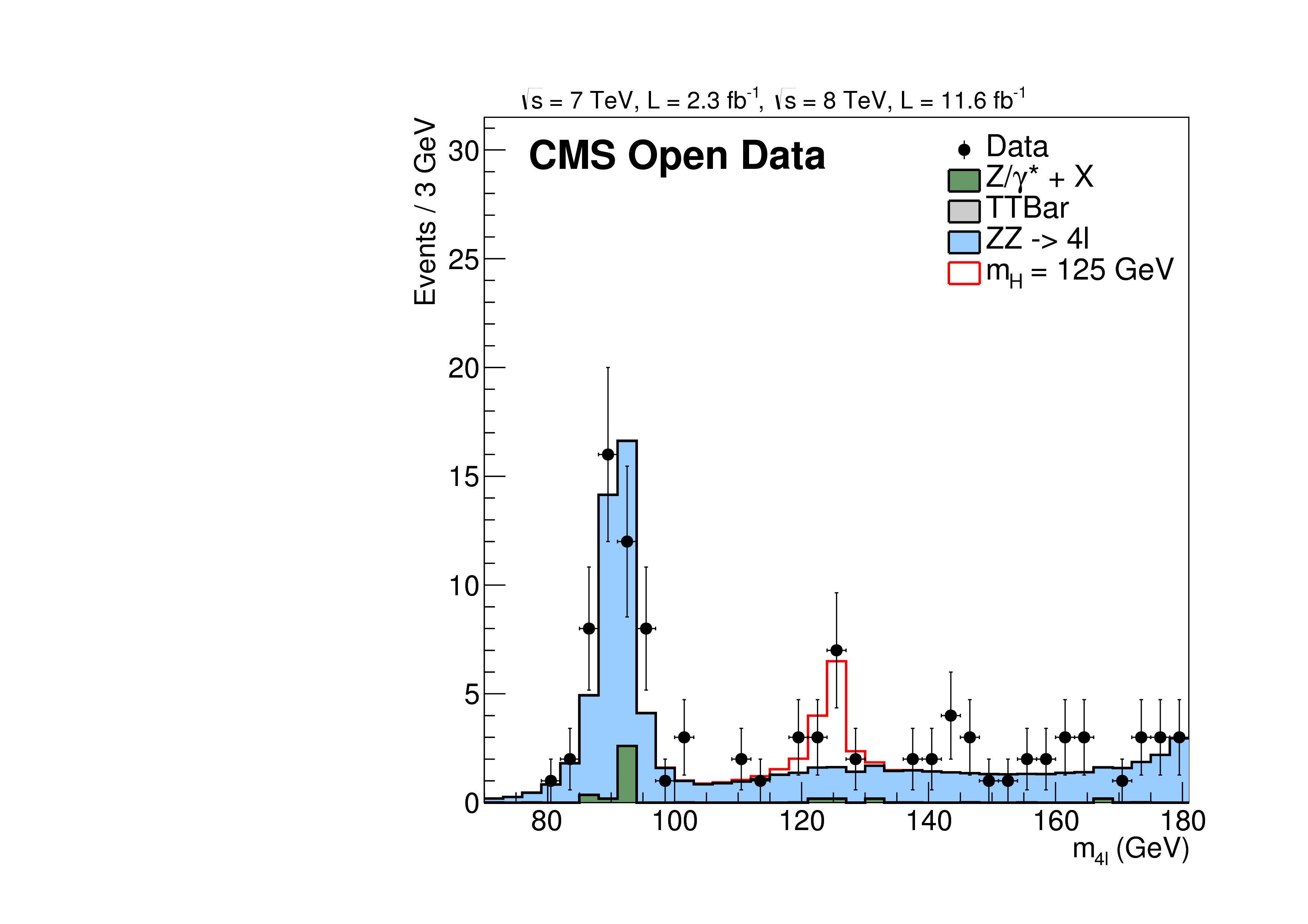
This research level example is a strongly simplified reimplementation of parts of the original CMS Higgs to four lepton analysis published in Phys.Lett. B716 (2012) 30-61, arXiv:1207.7235.
The published reference plot which is being approximated in this example is https://inspirehep.net/record/1124338/files/H4l_mass_3.png. Other Higgs final states (e.g. Higgs to two photons), which were also part of the same CMS paper and strongly contributed to the Higgs boson discovery, are not covered by this example.
The example consists of different levels of complexity. The highest level of this example addresses users who feel they have at least some minimal understanding of the content of this paper and of the meaning of this reference plot, which can be reached via (separate) educational exercises. The lower levels might also be interesting for educational applications. The example requires a minimal acquaintance with the linux operating system and the ROOT analysis tool.
The example uses legacy versions of the original CMS data sets in the CMS AOD, which slightly differ from the ones used for the publication due to improved calibrations. It also uses legacy versions of the corresponding Monte Carlo simulations, which are again close to, but not identical to, the ones in the original publication. These legacy data and MC sets listed below were used in practice, exactly as they are, in many later CMS publications.
Since according to the CMS Open Data policy the fraction of data which are public (and used here) is only 50% of the available LHC Run I samples, the statistical significance is reduced with respect to what can be achieved with the full dataset. However, the original paper Phys.Lett. B716 (2012) 30-61, arXiv:1207.7235, was also obtained with only part of the Run I statistics, roughly equivalent to the luminosity of the public sets, but with only partial statistical overlap.
The provided analysis code recodes the spirit of the original analysis and recodes many of the original cuts on original data objects, but does not provide the original analysis code itself. Also, for the sake of simplicity, it skips some of the more advanced analysis methods of the original paper. Nevertheless, it provides a qualitative insight about how the original result was obtained. In addition to the documented core results, the resulting root files also contain many undocumented plots which grew as a side product from setting up this example and earlier examples. The significance of the Higgs 'excess' is about 2 standard deviations in this example, while it was 3.2 standard deviations in this channel alone in the original publication. The difference is attributed to the less sophisticated background suppression. In more recent (not yet public) CMS data sets with higher statistics the signal is observed in a preliminary analysis with more than 5 standard deviations in this channel alone CMS-PAS-HIG-16-041.
The analysis strategy is the following: Get the 4mu and 2mu2e final states from the DoubleMuParked datasets and the 4e final state from the DoubleElectron dataset. This avoids double counting due to trigger overlaps. All MC contributions except top use data-driven normalization: The DY (Z/gamma^*) contribution is scaled to the Z peak. The ZZ contribution is scaled to describe the data in the independent mass range 180-600 GeV. The Higgs contribution is scaled to describe the data in the signal region. The (very small) top contribution remains scaled to the MC generator cross section.
Use with
The example uses legacy versions of the original CMS datasets in the AOD format, which slightly differ from the ones used for the original publication due to improved calibrations. It also uses legacy versions of the corresponding Monte Carlo simulations, which are again close to, but not identical to, the ones in the original publication. These legacy data and MC sets listed below were used in practice, exactly as they are, in many later CMS publications.
/DoubleElectron/Run2011A-12Oct2013-v1/AOD
/DoubleMu/Run2011A-12Oct2013-v1/AOD
/ZZTo4mu_mll4_7TeV-powheg-pythia6/Summer11LegDR-PU_S13_START53_LV6-v1/AODSIM
/ZZTo4e_mll4_7TeV-powheg-pythia6/Summer11LegDR-PU_S13_START53_LV6-v1/AODSIM
/ZZTo2e2mu_mll4_7TeV-powheg-pythia6/Summer11LegDR-PU_S13_START53_LV6-v1/AODSIM
/SMHiggsToZZTo4L_M-125_7TeV-powheg15-JHUgenV3-pythia6/Summer11LegDR-PU_S13_START53_LV6-v1/AODSIM
/DYJetsToLL_M-50_7TeV-madgraph-pythia6-tauola/Summer11LegDR-PU_S13_START53_LV6-v1/AODSIM
/DYJetsToLL_M-10To50_TuneZ2_7TeV-pythia6/Summer11LegDR-PU_S13_START53_LV6-v1/AODSIM
/TTTo2L2Nu2B_7TeV-powheg-pythia6/Summer11LegDR-PU_S13_START53_LV6-v1/AODSIM
/DoubleMuParked/Run2012B-22Jan2013-v1/AOD
/DoubleMuParked/Run2012C-22Jan2013-v1/AOD
/DoubleElectron/Run2012B-22Jan2013-v1/AOD
/DoubleElectron/Run2012C-22Jan2013-v1/AOD
/ZZTo4mu_8TeV-powheg-pythia6/Summer12_DR53X-PU_RD1_START53_V7N-v1/AODSIM
/ZZTo4e_8TeV-powheg-pythia6/Summer12_DR53X-PU_RD1_START53_V7N-v2/AODSIM
/ZZTo2e2mu_8TeV-powheg-pythia6/Summer12_DR53X-PU_RD1_START53_V7N-v2/AODSIM
/SMHiggsToZZTo4L_M-125_8TeV-powheg15-JHUgenV3-pythia6/Summer12_DR53X-PU_S10_START53_V19-v1/AODSIM
/TTbar_8TeV-Madspin_aMCatNLO-herwig/Summer12_DR53X-PU_S10_START53_V19-v2/AODSIM
Characteristics
10 files. 235.6 KiB in total.System details
Use this code with the CMS Open Data VM environmentCMSSW_5_3_32
How can you use this?
In addition to the instructions below which guide you through the example in detail, a github repository based on this original example is also provided. The root files needed for the Level 3 exercise can be found here.
There are four levels of increasing complexity for this example:
- Compare the provided final output plot mass4l_combine.pdf or mass4l_combine.png to the published one, keeping in mind the caveats mentioned in this record.
- Reproduce the final output plot from the predefined histogram files using a root macro (~few minutes - ~few hours, depending on setup and proficiency)
- if a ROOT version on the local computer compatible with ROOT 5.32/00 is running, use the local version (avoids installation of VM). Otherwise, follow the instructions in CMS 2011 Virtual Machines: How to install up to and including the command 'cmsenv', in order to install the VirtualBox and the CMS Open Data VM, and run ROOT there (the validation step with the Demo example may be skipped)
- if not already proficient in ROOT, consider doing a brief ROOT introductory tutorial in order to understand what the root macro will do
- create a new directory, e.g. rootfiles
mkdir rootfiles - switch to that directory
cd rootfilesand download the preproduced *.root histogram files given in this record for all relevant samples to this directory - Alternatively, on the command line in the directory
rootfiles, typewget http://opendata.web.cern.ch/record/5501/files/rootfilelist.txtand thenwget -i rootfilelist.txt - If you wish, you may look at the content of these files using ROOT: e.g. type
root, and on the root promt, typeTBrowser t, then double-click on the relevant file - download the root macro M4Lnormdatall.cc from this record into the same directory
- on the linux prompt, type
root -l M4Lnormdatall.cc - you will get the output plot on the screen
- either, on the ROOT canvas (picture) click
file->Quit ROOTor, on the root [] prompt, type.q - you will exit ROOT and find the output plot in mass4l_combined_user.pdf
- you can compare this plot with the plots provided in 1.
- Produce a root data input file from original data and MC files for one Higgs signal candidate and for the simulated Higgs signal with reduced statistics (for speed reasons) and reproduce the final output plot containing your own input using a root macro (~1 hour if Virtual machine is already installed, depending on internet connection and computer performance, up to ~few hours otherwise)
- if not already done, follow instructions for steps 1 and 2 in CMS 2011 Virtual Machines: How to install, including the installation of the demo analyzer
- in the
Demo/DemoAnalyzer/directory, which is created following Step 2: How to test and validate, replaceBuildFile.xmlby the version downloaded from this record - download HiggsDemoAnalyzer.cc from this record to the
Demo/Demoanalyzer/srcsubdirectory - in
Demo/DemoAnalyzer/, recompilescram b - download demoanalyzer_cfg_level3data.py (data example) and demoanalyzer_cfg_level3MC.py (Higgs simulation example)
- create datasets directory
mkdir datasetsand change to this directorycd datasets - download the 2012 JSON validation file from the corresponding record to this directory
- if not yet done at level 2, create the directory
rootfilesand download all the level 2 root files to this directory (see level 2) - run the two analysis jobs (one on data, one on MC, the input files are already predefined)
cmsRun demoanalyzer_cfg_level3data.pywill produce output fileDoubleMuParked2012C_10000_Higgs.rootcontaining 1 Higgs candidate from the datacmsRun demoanalyzer_cfg_level3MC.pywill produce output fileHiggs4L1file.rootcontaining the Higgs signal distributions with reduced statistics- move the two .root files above to the
rootfilesdirectory, together with the predefined files mv DoubleMuParked2012C_10000_Higgs.root rootfiles/.mv Higgs4L1file.root rootfiles/.- change directory
cd rootfilesand download the macro M4Lnormdatall_lvl3.cc to this directory - on the linux prompt, type
root -l M4Lnormdatall_lvl3.cc - you will get the output plot on the screen; the magenta Higgs signal histogram will now be the one you produced, and the one data event which you have selected will be shown as a blue triangle. All other parts of the plot are the same as in 2.
- either, on the ROOT canvas (picture) click
file->Quit ROOTor, on the root [] prompt, type.q - you will exit ROOT and find the output plot in mass4l_combined_user3.pdf
- Reproduce the full example analysis (up to ~1 month or more on single CPU with fast internet connection, depending on internet connection speed and computer performance)
- start by running level 3 and understand what you have done
- download demoanalyzer_cfg_level4data.py and demoanalyzer_cfg_level4MC.py from this record
- at this level, instead of running over a single file, you will run over so-called index files which contain chains of files
- download all the data index files for the datasets listed in List_indexfile.txt to the
datasetsdirectory (you can find the links to the datasets in this record) - download the 2011 JSON validation file to the
datasetsdirectory (in which you should already have the 2012 one) - download all the MC index files for the MC sets listed in
List_indexfile.txtto theMCsetsdirectory (after having created it) - edit the relevant demoanalyzer_cfg file and insert the index file you want; for data, make sure to use the correct JSON validation file in each case; set an output file name of your choice for each sample which you will recognise
- run the analysis job (
cmsRun demoanalyzer_cfg_level4...) sequentially on all the input samples listed inList_indexfile.txt, i.e. produce all root output files yourself. If you have access to a computer farm with local support for the installation of the CMS software (the Open Data team can only provide support for the single virtual machine mode), you may also run the analysis in parallel on different CPUs, correspondingly speeding up the result. - merge all the files from different index files of a dataset by using root tools
- If everything ran correctly, at this stage the content of your rootfiles should be identical to the one in the predefined rootfiles. If you don't want to run everything, you can also run only some of the datasets (but all events of all index files of a dataset must be treated and merged), and use the predefined ones for the others.
- go to 2., using your own root output files instead of the predefined ones, i.e. edit the file M4Lnormdatall.cc accordingly. If everything worked correctly you should get an output identical to mass4lcombine.pdf, but now using your own files.
Source code repository
A code repository based on the files attached to this record is also provided in:https://github.com/cms-opendata-analyses/HiggsExample20112012
Files and indexes
Disclaimer
These open data are released under the GNU General Public License v3.0.
Neither the experiment(s) ( CMS ) nor CERN endorse any works, scientific or otherwise, produced using these data.
This release has a unique DOI that you are requested to cite in any applications or publications.


